| Topic | Supported effect | Planning use |
|---|---|---|
| Explicit constraints | MPC is particularly effective in systems with constraints, such as maintaining safe operating conditions. | Choose MPC when the robot has limits it must never cross and you want them written into the controller. |
| Computation | MPC solves a constrained optimization problem in real time at every control step. Low-level robot drivers typically need updates on the order of 1 kHz, which is difficult for MPC to meet. | Settle the loop rate and the computing budget before committing to a formulation. |
| Model quality | MPC requires accurate system models, which can be challenging to obtain. | Budget time for modelling and validation, not only for tuning. |
| Tuning effort | PID controllers are favored for ease of implementation and tuning. | Keep PID for simple loops where limits and coupling are not the main problem. |
| Hard dynamics | PID can struggle with complex, multi-variable systems, especially those with significant delays or nonlinear dynamics. | Consider MPC, and a nonlinear model if the dynamics demand it, when coupling or delay dominates. |
These points come from a comparison of PID and MPC for high-speed robots and from a talk on fast MPC for robotic manipulators.
Model predictive control robotics applies a model of the robot to predict motion over a prediction horizon, optimizes the inputs under constraints, and applies only the first input before repeating. It suits constrained, demanding tasks; PID suits simple ones.
For where optimization-based control sits among other methods, see artificial intelligence in robotics. The sections below start with what choosing MPC changes in a project, then explain how the method works.
What choosing MPC changes in a robot project
MPC moves limits and foresight into the controller, and it moves cost into computation and modelling. A textbook from Middle Tennessee State University describes a model predictive controller as an optimal controller used in practical control applications, so the decisions below follow from that optimization step.
Constraints and planning in one loop
- Limits become part of the problem. Because constraints enter the optimization directly, the controller plans around them instead of reacting after they are violated. This is why MPC is described as particularly effective where safe operating conditions must be maintained.
- Planning and control share a loop. The optimizer looks across the horizon and then acts, so it behaves as a short-range planner and a controller at once. That makes it a natural fit for a robot following a path around an obstacle, where the next input depends on what lies ahead.
- Model accuracy sets the ceiling. The predictions are only as good as the model behind them. If the robot cannot be modelled well enough, the optimizer will plan confidently around the wrong dynamics.
- Compute becomes a design input. MPC requires significant computational resources, so the choice of processor, solver and model size belongs in the early design, not the final integration.
When the extra effort is not worth it
If a loop has no hard limits worth encoding and the dynamics are well behaved, MPC adds modelling and computing cost without a matching benefit. The same comparison notes that PID is favored where ease of implementation and tuning matter most. Choose MPC because the task has constraints or coupling, not because it is the more sophisticated option.
MPC versus PID on practical criteria
PID reacts to the error it sees now, while MPC reasons about the future the model predicts. A PID controller uses proportional, integral and derivative terms and is simple to implement and tune. MPC trades that simplicity for foresight and explicit limits.
- Tuning and implementation: PID wins. A small number of gains and a short implementation make it the sensible baseline for a single joint or speed loop.
- Constraints: MPC wins. Actuator limits and safe operating conditions can be stated as constraints, rather than handled by clamping outputs after the fact.
- Delays and nonlinear dynamics: MPC is the stronger candidate. PID can struggle with complex, multi-variable systems, especially those with significant delays or nonlinear dynamics.
- Computation and models: PID wins. MPC needs an accurate model and enough computing power to optimize at every step.
A practical pattern is to start with PID and move to MPC only when limits, delays or coupling between variables clearly defeat it. That keeps the first working version simple and gives MPC a measurable problem to solve.
Real-time limits on an onboard computer
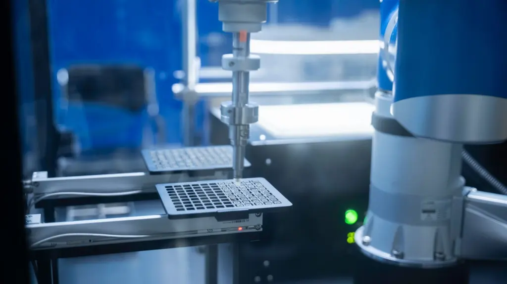
Whether MPC runs in real time on an onboard computer depends on how fast the loop must run and how heavy each optimization is. Research on fast MPC for robotic manipulators states that low-level drivers in robotic systems require input updates at high frequency, typically in the order of 1 kHz. It also calls that frequency difficult to meet for MPC because of its inherent computational complexity.
The reason is structural. MPC solves a constrained optimization problem in real time at every control step, so the solve time sets the achievable loop rate. A longer horizon, a richer model or more constraints all enlarge that problem.
- Fix the rate first. Decide the update rate the robot’s drivers actually need before choosing the horizon and model detail.
- Treat solve time as a budget. If the optimization cannot finish within a control step on the target computer, simplify the model or the horizon rather than hoping the hardware copes.
- Expect no universal yes. The evidence points to a computational challenge to be engineered around, not a guarantee, so test on the real onboard hardware.
Nonlinear MPC and published robot examples
You need nonlinear MPC when the robot’s dynamics are too nonlinear for a linear model to predict usefully. The earlier comparison notes that PID can struggle with non-linear dynamics, and MPC lets you place the nonlinearity in the prediction model itself.
An industrial robot in 2000
A paper published in 2000 at the Robotics 2000 conference, Model Predictive Control for Industrial Robots, states that the predictive model used is non-linear. It shows that nonlinear predictive models were already being applied to industrial manipulators well before today’s faster computers.
Legged robots and two planning levels
Legged locomotion is a demanding case. The Notre Dame ROAM lab notes that control of legged locomotion is often challenging because of the hybrid nature of the dynamics and the high-dimensional state. Its receding-horizon approach uses two planning levels: short-term whole-body dynamics and a long-term simplified template such as a linear inverted pendulum.
The practical lesson is that a full nonlinear model does not have to cover the whole horizon. Splitting detail between near and far futures is one way to keep a hard problem tractable.
How the MPC formulation works
MPC works by repeating a short cycle at every control step. The textbook formulation uses N as the prediction horizon, and the controller optimizes a sequence of future inputs over that span. The Middle Tennessee State University chapter then applies only the first of those inputs.
- Measure or estimate the current state of the robot.
- Predict the robot’s behaviour over the horizon using the model.
- Optimize the input sequence subject to the constraints.
- Apply the first control input to the system.
- Update the state and repeat the whole cycle.
Discarding the rest of the plan and re-solving is what makes the method a receding-horizon controller. It lets the robot correct for disturbances and model error at the next step, because the next solve starts from what actually happened.
For linear models with a quadratic cost and linear constraints, each solve is a quadratic program. In the textbook example, the MPC solver starts to solve the quadratic optimization problem in order to perform the control, and the example code uses cvxpy. Nonlinear MPC keeps the same cycle but solves a harder nonlinear problem each step, which is why its computing cost deserves attention early.
Setting up and tuning in practice
Setup is mostly a matter of deciding what the controller must respect and how much computing it can spend. The choices below follow from the evidence above and keep the work focused.
- Write the limits down first. List the actuator and safety limits the robot must honour, since these are what justify MPC over PID.
- Pick the simplest model that predicts well. A linear model keeps each solve a quadratic program; move to a nonlinear model only when the dynamics demand it.
- Choose the horizon against the solve time. The textbook defines the horizon as N but gives no default length, so set it by testing the trade between foresight and computing cost on the target hardware.
- Check the loop rate on the real computer. Confirm that each solve fits inside a control step before tuning anything else.

If the task is hard to model, a learned approach may be a better fit, and imitation learning robotics takes a different route to the same control problem by learning from demonstrations. Readers weighing control against other planning approaches can read how do robots make decisions for the broader context.
Frequently asked questions
What does N mean in the MPC formulation?
N is the prediction horizon, the span over which the controller predicts and optimizes future inputs. The textbook source gives the symbol and its role but no default length.
Which tool does the textbook example use for the optimization?
The example code in the Middle Tennessee State University chapter uses cvxpy to solve the quadratic optimization problem at each step.
How does a legged-robot MPC handle a long horizon?
The Notre Dame ROAM lab describes a planner that uses increasingly coarse time steps and relaxed constraints along the horizon, alongside a simplified long-term template.
Is MPC an optimal controller?
Yes. The textbook describes a model predictive controller as an optimal controller used in practical control applications, one that also takes system constraints into account.